Architecture

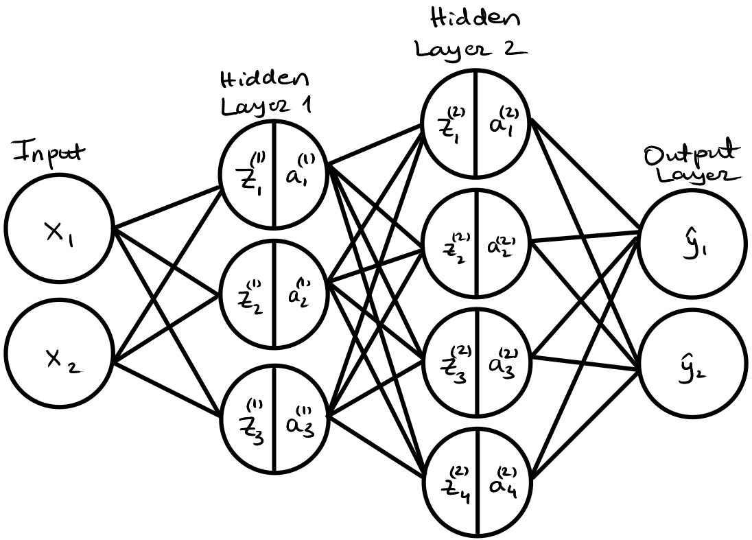
Below is the same example of a simple neural network with two-dimensional inputs, two hidden layers with 3 and 4 neurons respectively, and two-dimensional outputs.

Forward Pass in Matrix Notation

Layer 1 (Hidden Layer)

$$ z_i^{(1)} = b_i^{(1)} + \sum_j w_{ij}^{(1)} x_j \\ a^{(1)}_i = \tanh \left(z^{(1)}_i \right) $$

In Matrix form:

$$ \mathbf{z}^{(1)} = \mathbf{W}^{(1)}\mathbf{x} + \mathbf{b}^{(1)} \\[0.2cm] \mathbf{a}^{(1)} = \tanh \left( \mathbf{z}^{(1)} \right) $$

where $\mathbf{W}^{(1)} \in \mathbb{R}^{3\times2}$, $\mathbf{b}^{(1)} \in \mathbb{R}^{3\times1}$, $\mathbf{x} \in \mathbb{R}^{2\times1}$. The $\tanh$ is applied element wise.

Layer 2 (Hidden Layer)

$$ z_k^{(2)} = b_k^{(2)} + \sum_i w_{ki}^{(2)} a^{(1)}_i \\ a^{(2)}_k = \tanh \left(z^{(2)}_k \right) $$

In matrix form:

$$ \mathbf{z}^{(2)} = \mathbf{W}^{(2)}\mathbf{a}^{(1)} + \mathbf{b}^{(2)} \\[0.2cm] \mathbf{a}^{(2)} = \tanh \left( \mathbf{z}^{(2)} \right) $$

where $\mathbf{W}^{(2)} \in \mathbb{R}^{4\times3}$, $\mathbf{b}^{(2)} \in \mathbb{R}^{4\times1}$, $\mathbf{a}^{(1)} \in \mathbb{R}^{3\times1}$. The $\tanh$ is applied element wise.

Layer 3 (Output Layer)

$$ \hat{y}_l = b_l^{(3)} + \sum_k w^{(3)}_{lk}a_k^{(2)} \\ $$

In matrix form:

$$ \hat{\mathbf{y}} = \mathbf{W}^{(3)}\mathbf{a}^{(2)} + \mathbf{b}^{(3)} $$

where $\mathbf{W}^{(3)} \in \mathbb{R}^{2\times4}$, $\mathbf{b}^{(3)} \in \mathbb{R}^{2\times1}$, $\mathbf{a}^{(2)} \in \mathbb{R}^{4\times1}$.

Backward Pass in Matrix Notation

Layer 3 Parameters

$$ \frac{\partial L}{\partial b^{(3)}_{m}} = 2(\hat{y}_m - y_m) $$

$$ \frac{\partial L}{\partial \mathbf{b}^{(3)}} = \boldsymbol{\delta}^{(3)} $$

$$ \frac{\partial L}{\partial w^{(3)}_{mn}} = 2(\hat{y}_m - y_m) a^{(2)}_n $$

$$ \frac{\partial L}{\partial \mathbf{W}^{(3)}} = \boldsymbol{\delta}^{(3)} \left(\mathbf{a}^{(2)}\right)^\top $$

where $\boldsymbol{\delta}^{(3)} = 2(\hat{\mathbf{y}} - \mathbf{y})$. This is known as the error signal, representing the gradient of the loss function with respect to a layer (in this case the output layer). $\boldsymbol{\delta}^{(3)} \in \mathbb{R}^{2\times1}$, $\left(\mathbf{a}^{(2)}\right)^\top \in \mathbb{R}^{1\times4}$, $\frac{\partial L}{\partial \mathbf{W}^{(3)}} \in \mathbb{R}^{2\times4}$, $\frac{\partial L}{\partial \mathbf{b}^{(3)}} \in \mathbb{R}^{2\times1}$.

Layer 2 Parameters

$$ \frac{\partial L}{\partial b^{(2)}_{m}} = \sum_l 2(\hat{y}_l - y_l) w^{(3)}_{lm} \left (1-\tanh \left(z_m^{(2)}\right )^2 \right) = \left (1-\tanh \left(z_m^{(2)}\right )^2 \right) \sum_l 2(\hat{y}_l - y_l) w^{(3)}_{lm} $$

$$ \frac{\partial L}{\partial w^{(2)}_{mn}} = \sum_l 2(\hat{y}_l - y_l) w^{(3)}_{lm} \left (1-\tanh \left(z_m^{(2)}\right )^2 \right) a^{(1)}_n = \left (1-\tanh \left(z_m^{(2)}\right )^2 \right) a^{(1)}_n \sum_l 2(\hat{y}_l - y_l) w^{(3)}_{lm} $$

In matrix form:

$$ \frac{\partial L}{\partial \mathbf{b}^{(2)}} = \sigma'\left(\mathbf{z}^{(2)}\right) \odot \left( \left(\mathbf{W}^{(3)}\right)^\top \boldsymbol{\delta}^{(3)} \right) = \boldsymbol{\delta}^{(2)} $$

$$ \frac{\partial L}{\partial \mathbf{W}^{(2)}} = \left[ \sigma'\left(\mathbf{z}^{(2)}\right) \odot \left( \left(\mathbf{W}^{(3)}\right)^\top \boldsymbol{\delta}^{(3)} \right) \right] \left(\mathbf{a}^{(1)}\right)^\top = \boldsymbol{\delta}^{(2)} \left(\mathbf{a}^{(1)}\right)^\top $$

$\boldsymbol{\delta}^{(2)} \in \mathbb{R}^{4\times1}$, $\left(\mathbf{a}^{(1)}\right)^\top \in \mathbb{R}^{1\times3}$, $\frac{\partial L}{\partial \mathbf{W}^{(2)}} \in \mathbb{R}^{4\times3}$, $\frac{\partial L}{\partial \mathbf{b}^{(2)}} \in \mathbb{R}^{4\times1}$. The $\sigma'$ function is the derivative of the activation function. The $\odot$ indicates the Hadamard product, which is element-wise multiplication.

Layer 1 Parameters

$$ \frac{\partial L}{\partial b^{(1)}_{m}} = \sum_l 2(\hat{y}_l - y_l) \sum_k w^{(3)}_{lk} \left (1-\tanh \left(z_k^{(2)}\right )^2 \right) w_{km}^{(2)} \left( 1-\tanh\left( z^{(1)}_m \right)^2 \right) $$

$$ \frac{\partial L}{\partial w^{(1)}_{mn}} = \sum_l 2(\hat{y}_l - y_l) \sum_k w^{(3)}_{lk} \left (1-\tanh \left(z_k^{(2)}\right )^2 \right) w_{km}^{(2)} \left( 1-\tanh\left( z^{(1)}_m \right)^2 \right) x_n $$

In matrix form, these become:

$$ \frac{\partial L}{\partial \mathbf{b}^{(1)}} = \sigma'\left(\mathbf{z}^{(1)}\right) \odot \left( \left(\mathbf{W}^{(2)}\right)^\top \left[ \sigma'\left(\mathbf{z}^{(2)}\right) \odot \left( \left(\mathbf{W}^{(3)}\right)^\top \boldsymbol{\delta}^{(3)} \right) \right] \right) = \sigma'\left(\mathbf{z}^{(1)}\right) \odot \left( \left(\mathbf{W}^{(2)}\right)^\top \boldsymbol{\delta}^{(2)} \right) = \boldsymbol{\delta}^{(1)} $$

$$ \frac{\partial L}{\partial \mathbf{W}^{(1)}} = \left[ \sigma'\left(\mathbf{z}^{(1)}\right) \odot \left( \left(\mathbf{W}^{(2)}\right)^\top \left[ \sigma'\left(\mathbf{z}^{(2)}\right) \odot \left( \left(\mathbf{W}^{(3)}\right)^\top \boldsymbol{\delta}^{(3)} \right) \right] \right) \right] \mathbf{x}^\top = \left[ \sigma'\left(\mathbf{z}^{(1)}\right) \odot \left( \left(\mathbf{W}^{(2)}\right)^\top \boldsymbol{\delta}^{(2)} \right) \right] \left(\mathbf{x}\right)^\top = \boldsymbol{\delta}^{(1)} \mathbf{x}^\top $$

$\boldsymbol{\delta}^{(1)} \in \mathbb{R}^{3\times1}$, $\mathbf{x}^\top \in \mathbb{R}^{1\times2}$, $\frac{\partial L}{\partial \mathbf{W}^{(1)}} \in \mathbb{R}^{3\times2}$, $\frac{\partial L}{\partial \mathbf{b}^{(1)}} \in \mathbb{R}^{3\times1}$.

Generalized Equations

As you can see from the equations above, we always end up with essentially the same equations. We can generalize the derivative with respect to all layers as

$$ \boldsymbol{\delta}^{(q)} = \sigma'\left(\mathbf{z}^{(q)}\right) \odot \left( \left(\mathbf{W}^{(q+1)}\right)^\top \boldsymbol{\delta}^{(q+1)} \right) $$

$$ \frac{\partial L}{\partial \mathbf{b}^{(q)}} = \boldsymbol{\delta}^{(q)} $$

$$ \frac{\partial L}{\partial \mathbf{W}^{(q)}} = \boldsymbol{\delta}^{(q)} \left(\mathbf{a}^{(q-1)}\right)^\top $$

Row Vector Input and Batching

Typically, in packages like PyTorch, it is expected that the input is of shape $N \times D$ where $N$ is the number of samples in a batch/mini-batch and D is the dimensionality. The equations then become:

Forward Pass

$$ \mathbf{Z}^{(q)} = \mathbf{A}^{(q-1)} \left(\mathbf{W}^{(q)}\right)^\top \oplus \left(\mathbf{b}^{(q)}\right)^\top \\[0.2cm] \mathbf{A}^{(q)} = \tanh\left(\mathbf{Z}^{(q)}\right) $$

where $\mathbf{A}^{(q-1)} \in \mathbb{R}^{N\times D}$, $\left(\mathbf{W}^{(q)}\right)^\top \in \mathbb{R}^{D\times E}$ (where $E$ is the number of neurons in layer $q$), and $\left(\mathbf{b}^{(q)}\right)^\top \in \mathbb{R}^{1\times E}$. Note $\mathbf{A}^{(0)} = \mathbf{X}$, and that the output layer has no activation function. Also note that $\oplus$ indicates that the bias row vector is added for each row of the resulting matrix.

Loss

$$ L = \frac{1}{N}\mathbf{1}_N^\top \left[ (\hat{\mathbf{Y}} - \mathbf{Y}) \odot (\hat{\mathbf{Y}} - \mathbf{Y}) \right] \mathbf{1}_E $$

where $L \in \mathbb{R}$. The predictions $\hat{\mathbf{Y}} \in \mathbb{R}^{N\times E}$ are summed over the batch dimension with $\mathbf{1}_N^\top$ and summed over the output dimensions with $\mathbf{1}_E$ to get a scalar loss value. Then we divide by $N$ because we want to get an average of the loss calculated for the mini-batch of training data.

Backward Pass

The output layer error signal:

$$ \boldsymbol{\Delta}^{(3)} = \frac{2}{N}(\hat{\mathbf{Y}} - \mathbf{Y}) $$

where $\boldsymbol{\Delta}^{(3)} \in \mathbb{R}^{N\times 2}$ (in this case we have 2 outputs).

The hidden layer error signal is propagated backward as:

$$ \boldsymbol{\Delta}^{(q)} = \left(\boldsymbol{\Delta}^{(q+1)} \mathbf{W}^{(q+1)}\right) \odot \sigma'\left(\mathbf{Z}^{(q)}\right) $$

The parameter gradients are:

$$ \frac{\partial L}{\partial \mathbf{W}^{(q)}} = \left(\boldsymbol{\Delta}^{(q)}\right)^\top \mathbf{A}^{(q-1)} $$

$$ \frac{\partial L}{\partial \mathbf{b}^{(q)}} = \mathbf{1}_N^\top \boldsymbol{\Delta}^{(q)} $$

where $\mathbf{1}_N^\top \boldsymbol{\Delta}^{(q)}$ sums $\boldsymbol{\Delta}^{(q)}$ over the batch dimension.

Updating Parameters with Gradient Descent

With the equations above, we find the gradient of the loss function with respect to all of the parameters of the neural network. The gradient gives us the direction of steepest ascent, i.e. it points in the direction of increasing loss. As the goal of training is to decrease the loss, we need to go in the opposite direction of the gradient. Therefore, to update the full parameter vector, containing all parameters in the model, we need to do:

$$ \boldsymbol{\theta}_{i+1} = \boldsymbol{\theta}_{i} - \gamma(\nabla L(\boldsymbol{\theta}_{i})) $$

where $i$ indicates the current iteration and $i+1$ indicates the updated parameters to be used in the next iteration of training. $\gamma$ indicates the learning rate, i.e. how we scale the calculated gradient. For example, to update the weights in the 3rd layer, we can do

$$ \mathbf{W}^{(3)}_{i+1} = \mathbf{W}^{(3)}_{i} - \gamma \left.\frac{\partial L}{\partial \mathbf{W}^{(3)}}\right|_{\boldsymbol{\theta}_i} $$

where ${\boldsymbol{\theta}_i}$ means the partial derivative of the loss with respect to $\mathbf{W}^{(3)}$ is evaluated with the current parameters at step $i$.

The above equations represent Stochastic Gradient Descent (SGD) when using mini-batches, which is a simple method to update the model parameters. More complex optimization algorithms include momentum and other parameters in order to increase training efficiency.